Training, debugging and running time series forecasting models with the GluonTS toolkit on Amazon SageMaker

Time series forecasting is an approach to predict future data values by analyzing the patterns and trends in past observations over time. Organizations across industries require time series forecasting for a variety of use cases, including seasonal sales prediction, demand forecasting, stock price forecasting, weather forecasting, financial planning, and inventory planning.

Various cutting edge algorithms are available for time series forecasting, such as DeepAR, the seq2seq family, and LSTNet (Long- and Short-term Time-series network). The machine learning (ML) process for time series forecasting is often time-consuming, resource intensive, and requires comparative analysis across multiple parameter combinations and datasets to reach the required precision and accuracy with your models. To determine the best model, developers and data scientists need to:

1. Select algorithms and hyperparameters.
2. Build, configure, train, and tune models.
3. Evaluate these models and compare metrics captured at training and evaluation time.
4. Visualize results.
5. Repeat the preceding steps multiple times before choosing the optimal model.

The infrastructure management associated with the scaling required at training time for such an iterative process may lead to undifferentiated heavy lifting for the developers and data scientists involved.

In this post and the associated notebook, we show you how to address these challenges by providing an approach with detailed steps to set up and run time series forecasting models at scale using Gluon Time Series (GluonTS) on Amazon SageMaker. GluonTS is a Python toolkit for probabilistic time series modeling, built around Apache MXNet. GluonTS provides utilities for loading and iterating over time series datasets, state-of-the-art models ready to be trained, and building blocks to define your own models and quickly experiment with different solutions.

Solution overview

We first show you how to set up GluonTS on SageMaker using the MXNet estimator, then train multiple models using SageMaker Experiments, use SageMaker Debugger to mitigate suboptimal training, evaluate model performance, and finally generate time series forecasts. We walk you through the following steps:

1. Prepare the time series dataset.
2. Create the algorithm and hyperparameters combinatorial matrix.
3. Set up the GluonTS training script.
4. Set up a SageMaker experiment and trials.
5. Create the MXNet estimator.
6. Set up an experiment with Debugger enabled to automatically stop suboptimal jobs.
7. Train and validate models.
8. Evaluate metrics and select a winning candidate.
9. Run time series forecasts.

Prerequisites

Before getting started, you must set up your SageMaker notebook instance and install the required packages. Complete the following steps:

1. Onboard to Amazon SageMaker Studio with the Quick start procedure.
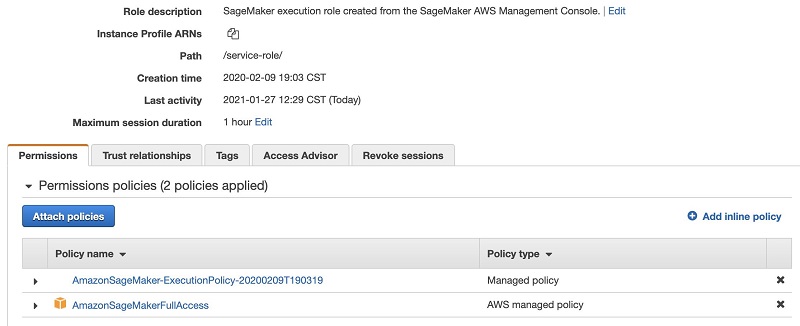
2. When you create an AWS Identity and Access Management (IAM) role to the notebook instance, be sure to specify access to Amazon Simple Storage Service (Amazon S3). You can choose any S3 bucket or specify the S3 bucket you want to enable access to. You can use the AWS-managed policies AmazonSageMakerFullAccess to grant general access to SageMaker services.

3. When the user is created and active, choose Open Studio.

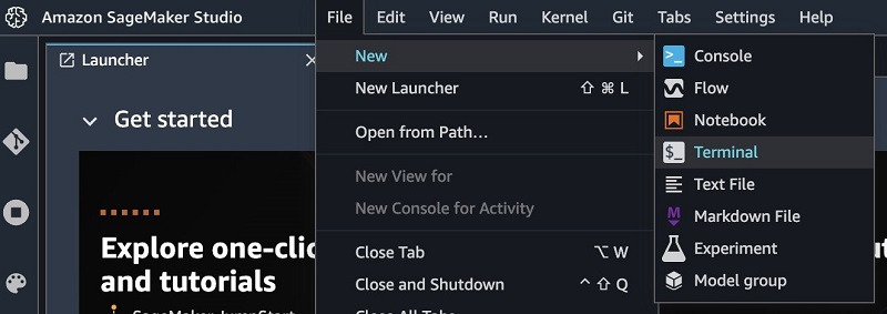
4. On the Studio landing page, on the File drop-down menu, choose New.
5. Choose Terminal.

6. In the terminal, enter the following code:

   git clone https://github.com/aws-samples/amazon-sagemaker-gluonts-timeseriesforecasting-with-debuggerandexperiments

7. Open the notebook by choosing Amazon SageMaker GluonTS time series forecasting.ipynb
8. Install the required packages by entering the following code:

   ! pip install gluonts
   ! pip install --upgrade sagemaker
   ! pip install sagemaker-experiments
   ! pip install --upgrade smdebug-rulesconfig

Preparing the time series dataset

For this post, we use the individual household electric power consumption dataset. (Dua, D. and Karra Taniskidou, E. (2017). UCI Machine Learning Repository. Irvine, CA: University of California, School of Information and Computer Science.) The usage data is aggregated hourly.

Let’s download and store the usage data as a DataFrame:

import pandas as pd
url = "https://raw.githubusercontent.com/aws-samples/amazon-forecast-samples/master/notebooks/common/data/item-demand-time.csv"
df = pd.read_csv(url, header=None, names=["date", "usage", "client"])

Define the S3 bucket and folder locations to store the test and training data. This should be within the same Region as the notebook instance, training, and hosting.

Now let’s divide the raw data into train and test samples and save them in their respective S3 folder locations using the Pandas DataFrame query function. We can check first few entries of the train and test dataset. Both datasets should have the same fields, as in the following code:

df_train = df.query('date <= "2014-31-10 11:00:00"').copy()
df_train.to_csv("train.csv")
s3_client.upload_file("train.csv", "glutonts-electricity", pref+"/train.csv")
df_train.head()

df_test = df.query('date >= "2014-1-11 12:00:00"').copy()
df_test.to_csv("test.csv")
s3_client.upload_file("test.csv", "glutonts-electricity", pref+"/test.csv")
df_test.head()

Creating the algorithm and hyperparameters combinatorial matrix

GluonTS comes with pre-built probabilistic forecasting models. Instead of simply predicting a single point estimate, probabilistic forecasting assigns a probability to every outcome. GluonTS provides a number of ready to use algorithm packages for training probabilistic forecasting models. When you select an algorithm, you can configure the hyperparameters to control the learning process during model training.

SageMaker supports bring your own model using Script mode. You can use SageMaker to train and deploy a model using custom MXNet code. The Amazon SageMaker Python SDK MXNet estimators and models and the SageMaker open-source MXNet container make writing a MXNet script and running it in SageMaker easier.

In this post, we train using four different models from the GluonTS toolkit: 

DeepAR – A supervised learning algorithm for forecasting scalar time series using Recurrent Neural Networks (RNN)

SFeedFwd (Simple Feedforward) – A supervised learning algorithm where information moves in only one direction—forward—from the input nodes, through the hidden nodes (if any), and to the output nodes in the forward direction

LSTNet – A multivariate time series forecasting model that uses the combination of Convolution Neural Network (CNN) and the RNN to find short-term local dependency patterns among variables and then find long-term patterns for time series trends

seq2seq (sequence-to-sequence learning) – A family of architectures; for this post we use the MQCNNEstimator of the seq2seq family to set up our training

All these algorithms are already part of GluonTS; we use it to quickly iterate and experiment over different models.

A trainer defines how a network is going to be trained. Let’s define a trainer object using a Pandas DataFrame that has the base list of algorithms, different epochs, learning rate, and hyperparameter combinations that we want to define for our training runs. We use the product function to derive combinations of these parameters from the base set into separate rows in the DataFrame. Each row corresponds to a training job configuration that we subsequently pass to the MXNet estimator to run the training job. See the following code:

import pandas as pd
d = {'epochs': [5, 10, 15, 20], 'algo': ["DeepAR", "SFeedFwd", "lstnet", "seq2seq"], 'num_batches_per_epoch': [10, 15, 20, 25], 'learning_rate':[1e-2, 1e-3, 1e-3, 1e-3], 'hybridize':[False, True, True, True]}
df_hps = pd.DataFrame(data=d)
df_hps['prediction_length'] = [30, 60, 75, 100]

from itertools import product

prod = product(df_hps['epochs'].unique(), df_hps['algo'].unique(), df_hps['num_batches_per_epoch'].unique(), df_hps['learning_rate'].unique(), df_hps['hybridize'].unique(), df_hps['prediction_length'].unique())
df_hps_combo = pd.DataFrame([list(p) for p in prod],
               columns=list(['epochs', 'algo', 'num_batches_per_epoch', 'learning_rate', 'hybridize', 'prediction_length']))
df_hps_combo['jobnumber'] = df_hps_combo.index

Setting up the GluonTS training script

We use a Python entry script to import the necessary GluonTS libraries, set up the GluonTS estimators using the model packages for our algorithms of interest, and pass in our algorithm and hyperparameter preferences from the MXNet estimator we set up in the notebook. The script uses the train and test data files we uploaded to Amazon S3 to create the corresponding GluonTS datasets for training and evaluation. When training is complete, the script runs an evaluation to generate metrics and store them using the SageMaker Debugger hook function, which we use to choose a winning model. For further analysis, the metrics are also available via the SageMaker trial component analytics (which we discuss later in this post). The model is then serialized for storage and future retrieval.

For more details, refer to the entry script available in the GitHub repo. From the accompanying notebook, you can also run the cell in Step 3 to review the script.

Setting up a SageMaker experiment

SageMaker Experiments automatically tracks the inputs, parameters, configurations, and results of your iterations as trials. You can assign, group, and organize these trials into experiments. SageMaker Experiments is integrated with SageMaker Studio, providing a visual interface to browse your active and past experiments, compare trials on key performance metrics, and identify the best-performing models. SageMaker Experiments comes with its own Experiments SDK, which makes the analytics capabilities easily accessible in SageMaker notebooks. Because SageMaker Experiments enables tracking of all the steps and artifacts that go into creating a model, you can quickly revisit the origins of a model when you’re troubleshooting issues in production or auditing your models for compliance verifications. You can create your experiment with the following code:

from smexperiments.experiment import Experiment
sagemaker_boto_client = boto3.client("sagemaker")

Experiment.create(
experiment_name=experiment_name,
description="Timeseries models",
sagemaker_boto_client=sagemaker_boto_client)

For each job, we define a new trial component within that experiment. Next we define an experiment config, which is a dictionary that we pass into the fit() method later on. This ensures that the training job is associated with that experiment and trial. For the full code block for this step, refer to the accompanying notebook.

Creating the MXNet estimator

You can run MXNet training scripts on SageMaker by creating an MXNet estimator. Before setting up the actual training runs with the parameter sweep, let’s test the MXNet estimator using a single set of an algorithm and hyperparameters, in this case DeepAR. See the following code:

import sagemaker
from sagemaker.mxnet import MXNet

mxnet_estimator = MXNet(entry_point='blog_train_algos.py',
                        role=sagemaker.get_execution_role(),
                        train_instance_type='ml.m5.large',
                        train_instance_count=1,
                        framework_version='1.7.0', 
                        py_version='py3',
                        hyperparameters={'bucket': bucket,
                            'seq': 10,
                            'algo': "DeepAR",             
                            'freq': "D", 
                            'prediction_length': 30, 
                            'epochs': 10,
                            'learning_rate': 1e-3,
                            'hybridize': False,
                            'num_batches_per_epoch': 10,
                         })

After specifying our estimator with all the necessary hyperparameters, we can train it using our training dataset. We train it by invoking the fit() method of the estimator. We pass the location of train and test data as well as the experiment configuration. The training algorithm returns a fitted model (or a predictor in GluonTS parlance) that we can use to construct forecasts. See the following code:

mxnet_estimator.fit({"train": s3_train_channel, "test": s3_test_channel}, 
                    experiment_config=experiment_config,
                    wait=False)

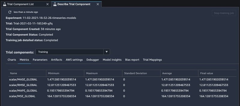
You can review the job parameters and metrics from the trial component view in SageMaker Studio (see the following screenshot).

Setting up an experiment with SageMaker Debugger enabled to automatically stop suboptimal jobs

We ran a parameter sweep and created lots of different configurations when we ran the product function to generate the hyperparameters combinatorial matrix in the second step above. Doing so may produce parameter combinations that lead to suboptimal models. We can use SageMaker Debugger to tune our experiment. Debugger automatically captures data from the model training and provides built-in rules that check for conditions such as overfitting and vanishing gradients. We can then specify actions to automatically stop training jobs ahead of time that would otherwise produce low-quality models. Some of the models in our experiment use RNNs that can suffer from the vanishing gradient problem. We use the Debugger tensor variance rule, which allows us to specify an upper and lower bound on the gradient values. We also specify the action StopTraining, which stops a training job when the rule triggers. By default, Debugger collects data with an interval of 500 steps. For this post, our training dataset is small and our models only train for a few minutes, so we can decrease the save interval. We create a custom collection, where we collect gradients at an interval of 5:

mxnet_estimator.fit({"train": s3_train_channel, "test": s3_test_channel}, 
                    experiment_config=experiment_config,
                    wait=False)
from sagemaker.debugger import DebuggerHookConfig, CollectionConfig

debugger_hook_config = DebuggerHookConfig(
      collection_configs=[ 
          CollectionConfig(
                name="custom_collection",
                parameters={ "include_regex": "(.*gradient)(?!.*featureembedder)(.*weight)",
                             "start_step": "10",
                             "save_interval": "5"})])

We then define a new SageMaker experiment to run the trials based on the combinatorial matrix we created earlier. When the experiment is complete, we can determine how many seconds it ran. We then define a helper function to compute the billable seconds and how many training jobs were stopped automatically. This setup is especially useful if you run a parameter sweep with training jobs that train for hours. In our case, each job only trained for less than 10 minutes. Until the Debugger data is uploaded, fetched, and downloaded into the processing job, a few minutes may pass, so the potential cost reduction is less for smaller training jobs.

#name of experiment
timestep = datetime.now()
timestep = timestep.strftime("%d-%m-%Y-%H-%M-%S")
experiment_name = timestep + "-timeseries-models"

#create experiment
Experiment.create(
    experiment_name=experiment_name, 
    description="Timeseries models", 
    sagemaker_boto_client=sagemaker_boto_client)

See the accompanying notebook for the full code in this section.

Training and validating models

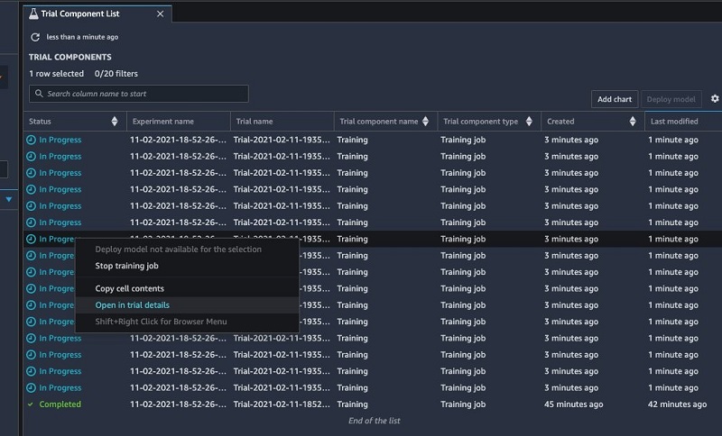
In a previous step, we trained one model. Now we iterate over all possible combinations of hyperparameters and algorithms that we generated using the product function with the SageMaker Debugger rules enabled to detect suboptimal training jobs and stop them automatically if the rule fails. A SageMaker experiment consists of multiple trials with a related objective. A trial consists of one or more trial components, such as a data preprocessing job and a training job. Each trial component within our experiment corresponds to one training job run. SageMaker Studio provides an experiments browser that you can use to view lists of experiments, trials, and trial components (see the following screenshot).

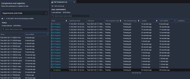
You can choose one of these entities to view detailed information about the entity or choose multiple entities for comparison (see the following screenshot).

For more information, see View Experiments, Trials, and Trial Components. For the code block for this step, refer to the accompanying notebook. If you would like to tune further, you can also run a hyperparameter tuning job. Amazon SageMaker automatic model tuning, also known as hyperparameter tuning, finds the best version of a model by running many training jobs on your dataset using the algorithm and ranges of hyperparameters that you specify. Please refer to the SageMaker documentation for an example.

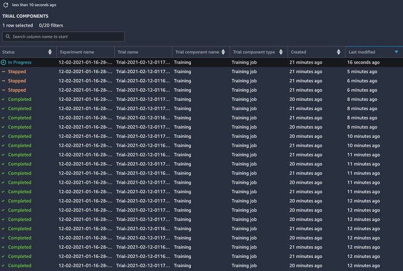
When our experiment completes its training run, we can check to see if any training jobs were stopped automatically. As we can see in the following screenshot, Debugger identified that the tensor variance of three jobs exceeded the gradient limits we set up in the rule and stopped them.

Evaluating metrics and selecting a winning candidate

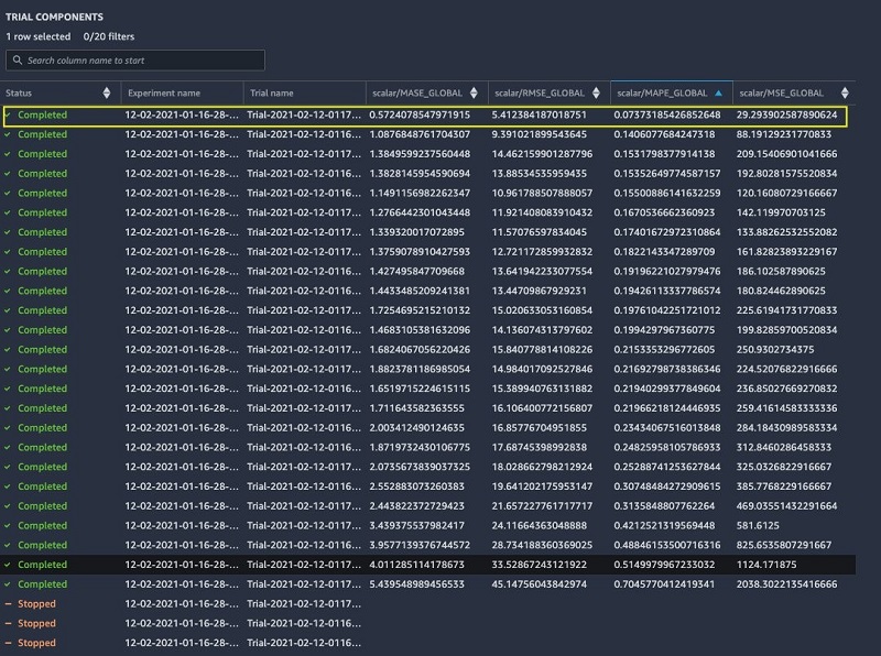
When the training jobs are running, we can use the experiments view in Studio or the ExperimentAnalytics module to track the status of our training jobs and their metrics. In the training script, we used the SageMaker Debugger function save_scalar to store metrics such as mean absolute percentage error (MAPE), mean squared error (MSE), and root mean squared error (RMSE) in the experiment. We can access the recorded metrics via the ExperimentAnalytics function and convert it to a Pandas DataFrame:

from sagemaker.analytics import ExperimentAnalytics

trial_component_analytics = ExperimentAnalytics(experiment_name=experiment_name)
df = trial_component_analytics.dataframe()
new_df = df[['epochs', 'learning_rate', 'hybridize', 'num_batches_per_epoch','prediction_length','scalar/MASE_GLOBAL - Min', 'scalar/MSE_GLOBAL - Min', 'scalar/RMSE_GLOBAL - Min', 'scalar/MAPE_GLOBAL - Min']]
mape_min = new_df['scalar/MAPE_GLOBAL - Min'].min()
df_winner = new_df[new_df['scalar/MAPE_GLOBAL - Min'] == mape_min]

Now let’s review the job summary and find the job with better forecasting accuracy. Different metrics define their own expectation function. The MAPE is a common statistical measure used for forecast accuracy. From our results matrix, let’s find the prediction job that has the lowest MAPE value to get the winning model. The following screenshot shows that the lowest MAPE in our run is 0.07373.

Download the winning model with the following code:

s3 = boto3.client("s3")
windir = "gluonts/blog-models/"+str(df_winner['jobnumber'].item())+"/"

def downloadDirectoryFroms3(bucket, windir):
    s3_resource = boto3.resource('s3')
    bucket = s3_resource.Bucket(bucket) 
    for obj in bucket.objects.filter(Prefix = windir):
        print(obj.key)
        if not os.path.exists(os.path.dirname(windir)):
            os.makedirs(os.path.dirname(windir))
        bucket.download_file(obj.key, obj.key) # save to same path


downloadDirectoryFroms3(bucket, windir)

Restore the predictor with the following code:

from gluonts.model.predictor import Predictor
path = pathlib.Path(windir)   
winning_predictor = Predictor.deserialize(path)

Running time series forecasts

When we use the GluonTS predictor to run our forecasts, we request predictions for the quantiles we’re interested in. A forecast at a specified quantile is used to provide a prediction interval, which is a range of possible values to account for forecast uncertainty. For example, a forecast at the 0.5 quantile estimates a value that is lower than the observed value 50% of the time. Our predictions return a QuantileForecast object that contains time series ordered in array for quantiles and mean. See the following code:

import matplotlib.pyplot as plt
from gluonts.dataset.common import ListDataset
plt.rcParams['figure.figsize'] = (20.0, 6.0)

# run forecast
startdate = '2014-11-01 01:00:00'
test_pred = ListDataset(
    [{"start": startdate, "target": raw_df.query('date >= "2014-11-01 01:00:00" and client == "client_12"').copy()['usage'], "item_id": 'client_12'}],
    freq = "1H"
)

pred = winning_predictor.predict(test_pred)
for test_entry, forecast in zip(test_pred, pred):
    print(forecast.start_date)
    plt.plot(pd.date_range(start=startdate, periods=30), pd.DataFrame.from_dict(test_entry['target'])[0][:30],color='b')
    plt.plot(pd.date_range(start=forecast.start_date, periods=df_winner['prediction_length'].item()), forecast.quantile(.3), color='r') #samples contain all 100 quantiles
    plt.plot(pd.date_range(start=forecast.start_date, periods=df_winner['prediction_length'].item()), forecast.quantile(.5), color='g') #samples contain all 100 quantiles
    plt.plot(pd.date_range(start=forecast.start_date, periods=df_winner['prediction_length'].item()), forecast.quantile(.7), color='k') #samples contain all 100 quantiles
    x=pd.date_range(start=forecast.start_date, periods=df_winner['prediction_length'].item()) #samples contain all 100 quantiles
    y=forecast.quantile(.1) 
    z=forecast.quantile(.9)
    plt.fill_between(x,y,z,color='g', alpha=0.3)
plt.xticks(rotation=30)
plt.legend(['Usage'], loc = 'lower left')
plt.show()

The blue line in the following forecasted plot represents the historical energy usage for a specific client, and the red, green, and black lines indicate the predicted energy usage at 30%, 50%, and 70% quantiles respectively for that client.

For more details, see the GluonTS Model Forecast module.

Conclusion

With SageMaker, it’s easy for every developer and data scientist to set up time series forecasting at scale using the MXNet estimator with the GluonTS toolkit. SageMaker removes the undifferentiated heavy lifting from every step of our ML process, automates infrastructure management, enables us to improve the training efficiency with SageMaker Debugger, and accelerates adoption of ML workflows from months to days. Try out the notebook from our post and let us know your comments and feedback.

References

For more information about GluonTS and algorithms like DeepAR, see the following:

• Elastic Machine Learning Algorithms in Amazon SageMaker
• DeepAR: Probabilistic forecasting with autoregressive recurrent networks
• GluonTS: Probabilistic and Neural Time Series Modeling in Python

About the Authors

Prem Ranga is an Enterprise Solutions Architect based out of Atlanta, GA. He is part of the Machine Learning Technical Field Community and loves working with customers on their ML and AI journey. Prem is passionate about robotics, is an Autonomous Vehicles researcher, and also built the Alexa-controlled Beer Pours in Houston and other locations.

Nathalie Rauschmayr is an Applied Scientist at AWS, where she helps customers develop deep learning applications.

Mona Mona is an AI/ML Specialist Solutions Architect based out of Arlington, VA. She works with the World Wide Public Sector team and helps customers adopt machine learning on a large scale. She is passionate about NLP and ML explainability areas in AI/ML.

Jana Gnanachandran is an Enterprise Solutions Architect at AWS, focusing on Data Analytics, AI/ML, and Serverless platforms. He helps AWS customers across numerous industries to design and build highly scalable, data-driven, analytical solutions to accelerate their cloud adoption. In his spare time, he enjoys playing tennis, 3D printing, and photography.