Artificial Intelligence
Deploy variational autoencoders for anomaly detection with TensorFlow Serving on Amazon SageMaker
Anomaly detection is the process of identifying items, events, or occurrences that have different characteristics from the majority of the data. It has many applications in various fields, like fraud detection for credit cards, insurance, or healthcare; network intrusion detection for cybersecurity; KPI metrics monitoring for critical systems; and predictive maintenance for in-service equipment. There are four main categories of techniques to detect anomalies: Classification, nearest neighbor, clustering, and statistical. In this post, we focus on a deep learning statistical anomaly detection approach using variational autoencoders.
Deep learning is a sub-field of machine learning (ML) and has been rapidly growing in the past few years. Due to its flexible structure and ability to learn non-linear relationships between data, deep learning models have been proven to be very powerful in solving different problems. An autoencoder is a type of neural network that can be used to learn hidden encoding of input data, which can be used for detecting anomalies. A variational autoencoder can be defined as being an autoencoder whose training is regularized to avoid overfitting and ensure that the latent space has good properties through a probabilistic encoder that enables the generative process.
To enable real-time predictions, you must deploy a trained ML model to an endpoint. Sometimes you may want to deploy more than one model at the same time. A standard practice is to deploy each model to a separate endpoint. Amazon SageMaker uses the TensorFlow Serving REST API to allow you to deploy multiple models to a single multi-model endpoint. Multi-model endpoints provide a scalable and cost-effective solution for deploying a large number of models. They use a shared TFS container that is enabled to host multiple models. This reduces hosting costs by improving endpoint utilization compared with using single-model endpoints. It also reduces deployment overhead because SageMaker manages loading models in memory and scaling them based on their traffic patterns.
In this post, we discuss the implementation of a variational autoencoder on SageMaker to solve an anomaly detection task. We also include examples of how to deploy multiple trained models to a single TensorFlow Serving multi-model endpoint. You can follow the code in the post to run the pipeline from beginning to end.
Dataset
The MNIST dataset is a large database of handwritten digits. It contains 60,000 training images and 10,000 testing images. They are small, 28×28 pixel, grayscale images between 0–9.
Variational autoencoder
An autoencoder is a type of artificial neural network used to learn efficient data coding in an unsupervised manner. An autoencoder has two connected networks:
- Encoder – Takes an input and converts it into a compressed knowledge representation in the bottleneck layer
- Decoder – Converts the compressed representation back to the original input
Standard autoencoders learn to generate compact representations of the input. One problem with autoencoders is overfitting, in which the data is reconstructed without any reconstruction loss, which leads to some points of the latent space giving meaningless content after they’re decoded. Another problem is that the latent space may not be continuous, which might cause the decoder to generate an unrealistic output because it doesn’t know how to deal with the region of latent space it hasn’t been seen before.
A variational autoencoder (VAE) provides a probabilistic manner for describing an observation in latent space. Compared with deterministic mappings used by an autoencoder for predictions, a VAE’s bottleneck layer provides a probabilistic Gaussian distribution of hidden vectors by predicting the mean and standard deviation of the distribution. A VAE’s latent spaces are continuous, allowing random sampling and interpolation. VAEs account for the variability of the latent space, which makes the model robust and able to achieve higher performance when compared with an autoencoder-based anomaly detection.
The following diagram illustrates this workflow.
Construct the problem
In this post, we use the MNIST dataset to construct an anomaly detection problem. For an anomaly detection problem, we have normal data as well as anomalies—the normal data is the majority and anomalies the minority. We train the VAE model on normal data, then test the model on anomalies to observe the reconstruction error. This technique is called semi-supervised because the model has only seen normal data during training. In real-world scenarios, we don’t necessarily have labeled anomalies; under such circumstances the semi-supervised method is especially useful. We can train the model to learn the pattern of normal data, so when anomalies happened, the model can identify the data that doesn’t fall into the pattern.
For our use case, we choose 1 and 4 as normal numbers and train the VAE model on the images from MNIST that contain 1 and 4. We choose 5 as the anomaly number and test the model on images with 5 in them to observe the reconstruction error.
Prepare the data
First, import the required packages and set up the SageMaker role and session. We import two files from the src folder: the config file defines the parameters to be used in the scripts, and the model_def contains the functions defining the VAE model. See the following code:
Next, let’s load the MNIST dataset from TensorFlow and reshape the data. We use train_x, train_y, test_x, and test_y, whose shapes are (60000, 28, 28, 1), (10000, 28, 28, 1), (60000, 10), and (10000, 10), respectively. The training dataset has 60,000 images and the testing dataset has 10,000 images. Each image is 28×28 pixels in greyscale. The dataset has 10 numbers from 0–9. See the following code:
Then we save the data locally for future usage. After the data is saved locally, we upload them to the default Amazon Simple Storage Service (Amazon S3) bucket. See the following code:
The MNIST dataset contains images with numbers 0-9. We selected 1 and 4 as normal numbers and 5 as the anomaly number. The next step is to separate the data accordingly into the normal and anomaly datasets for training and testing:
We now have an index of 12,585 normal images for training, 2,117 normal images for testing, and 6,313 anomaly images.
The next step is to prepare the data for training the model. For input data x, we convert the pixels to float and scale them to be between 0 and 1. For output data y, we one-hot encode the numbers into vectors of 0 and 1, with 1 representing the number. Then we use the index from the previous step to separate anomalies from normal data. See the following code:
Visualize the data
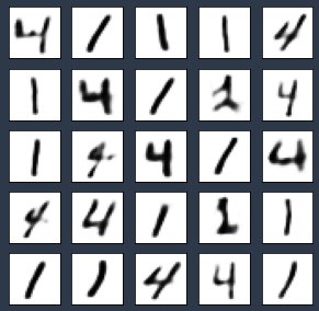
We plot the first 25 images of normal data and anomalies for double-checking:
The following image of the normal images shows 1 and 4.
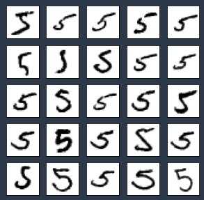
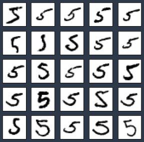
We plot the anomalies with the following code:
The image of the anomalies shows 5.
Train the model on SageMaker
SageMaker Script Mode allows you to train the model with the SageMaker pre-built containers for TensorFlow, PyTorch, and Apache MXNet and other popular frameworks on machines managed by SageMaker. For our use case, we use the TensorFlow 2.0 container provided by SageMaker. SageMaker training requires the data in Amazon S3 or an Amazon Elastic File System (Amazon EFS) or Amazon FSx for Lustre file system. For this post, we keep our data in Amazon S3. The training script (train.py) contains details of the training steps.
First, we set up a TensorFlow estimator object (estimator) for SageMaker hosted training. The key parameters for the estimator include the following:
- Hyperparameters – The hyperparameters for training the model
- entry_point – The path to the local Python source file, which should be run as the entry point to training
- instance_type – The type of instances used for training
- framework_version – The TensorFlow version you want to use for running your model training code
- py_version – The Python version you want to use for running your model training code
The estimator.fit sends train.py to be run on the TensorFlow container running on SageMaker hosted training instances. See the following code:
Download the model artifacts
After the model is trained, the model artifacts are saved in Amazon S3. We download the model artifacts from Amazon S3 to a local folder and extract them:
Deploy trained models to one endpoint
Our VAE has an encoder and a decoder. We use the encoder to get the condensed vector representations from the hidden layer, and the decoder to recreate the input. The encoder gives us the hidden layer distribution, from which we randomly sample condensed vector representations. These vector representations are passed through the decoder to generate the output, which is used to calculate the reconstruction error. In this section, we demonstrate how to deploy the encoder, decoder, as well as the whole VAE model to one single endpoint.
To deploy multiple models to a single TensorFlow Serving endpoint, the model artifacts need to be constructed in the following format:
└── multi
├── model1
│ └── <version number>
│ ├── saved_model.pb
│ └── variables
│ └── …
└── model2
└── <version number>
├── saved_model.pb
└── variables
└── …
Each folder in the model artifact contains a saved model and the related variables. They are deployed separately to a single endpoint.
Following the preceding format, we construct our output model artifacts in train.py, which contains five models:
- Variational autoencoders (
model/vae) - The model generating the mean of the hidden distributions (
model/encoder_mean) - The model generating the log variance of the hidden distributions (
model/encoder_lgvar) - The model generating the random samples from the hidden layer distribution defined by
encoder_meanandencoder_lgvar(model/encoder_sampler) - The decoder (
model/decoder)
The model/encoder_mean, model/encoder_lgvar, and model/encoder_sampler models combined serve as an encoder used to generate hidden vectors.
The following code shows our model structure:
└── model
├── vae
│ └── 1
│ ├── saved_model.pb
│ └── variables
│ └── …
├── encoder_mean
│ └── 2
│ ├── saved_model.pb
│ └── variables
│ └── …
├── encoder_lgvar
│ └── 3
│ ├── saved_model.pb
│ └── variables
│ └── …
├── encoder_sampler
│ └── 4
│ ├── saved_model.pb
│ └── variables
│ └── …
├── decoder
│ └── 5
│ ├── saved_model.pb
│ └── variables
│ └── …
├──test_loss.npy
└──train_loss.npy
Next, we use TensorFlow Serving to deploy all the models in the model artifact to a single endpoint. We provide the S3 path, SageMaker execution role, TensorFlow framework version, and the default model name to a TensorFlow model object. Then we deploy the model by calling model.deploy, during which we can set the hosting instance count as well as the instance type.
When model.deploy is called, on each instance, three steps occur:
- Start a Docker container optimized for TensorFlow Serving.
- Start a TensorFlow Serving process configured to run your model.
- Start an HTTP server that provides access to TensorFlow Server through the SageMaker
InvokeEndpoint
See the following code:
Now that the endpoint is created, we can get the predictor for each model by creating TensorFlow predictors. When creating the predictors, we provide the endpoint as well as the name of the model, which is the name of the folder that contains the model and its variables. The predictor object returned by the deploy function is ready to use to make predictions using the default model (vae in this example). See the following code:
Visualize the predictions
With the trained model, we can plot the prediction results for both normal and anomaly data. See the following code:
Generate input and prediction images for normal data with the following code:
The following image shows our inputs.
The following image shows the model predictions.
Generate input and prediction images for anomaly data with the following code:
The following image shows our inputs.
The following image shows the model predictions.
The results show that the model can recreate normal data very well. For anomaly data, the model reproduced certain features but not completely.
PCA of bottleneck layer vectors
Principal Component Analysis (PCA) is a dimension reduction method used to reduce the dimensionality of large datasets by transforming a large set of variables into a smaller one that still contains most of the information in the large set. The hidden (bottleneck) layer of the model provides the latent representations of the input data. These vectors contain compressed knowledge of the inputs. In the following code, we use PCA to find the principal components of the hidden vectors and visualize them to observe the distribution of the data:
The result shows that each number’s vectors cluster together. There is a little overlap between 4 and 5, which explains why some of the predictions of number 5 on the trained model preserve some features from 4.
Detect anomalies with reconstruction error
Reconstruction error is calculated using the reduced mean of the binary cross entropy. It tells us the difference between input images and reconstructed images. If the reconstruction error is high, it means there is a large difference between the input and the reconstructed output. Let’s calculate the reconstruction error for the train and test (normal and anomalies) datasets. In the following code: we take 2,000 data points from each dataset for a demonstration:
Next, we plot the reconstruction error for train normal and anomaly data:
From the graph, we have two observations:
- the reconstruction error for normal train and test is almost the same
- the reconstruction error for normal data is lower than the error for anomaly data.
Further statistics analysis shows that the average reconstruction loss for anomalies (225.75) is 171.39 higher than that of the normal data (54.36):
Evaluate the model performance
To evaluate the ability of the model to differentiate between normal data and anomalies, we set a threshold: when the reconstruction error is higher, we assign it as an anomaly, and when it’s lower, we assign it as normal data. To find the threshold, let’s look at statistical properties of the reconstruction error:
print(f'1, 99% Percentile of normal reconstruction loss is {np.percentile(train_normal_recon_loss, 1)}, {np.percentile(train_normal_recon_loss, 99)}')
print(f'4, 99% Percentile of abnormal reconstruction loss is {np.percentile(anomaly_recon_loss, 4)}, {np.percentile(anomaly_recon_loss, 99)}')
For normal data, 99% of the data has a reconstruction error lower than 120. For anomalies, 4% of the data has a reconstruction error lower than 126.94, which means 96% of the data has a reconstruction error higher than 126.94.
In this case, the 99 percentile of normal data reconstruction errors is a good threshold to use because it can separate the anomalies from normal data pretty well:
For ground truth data, we label the normal numbers (1 and 4) as True and anomalies (5) as False. For prediction labels, when reconstruction error is higher than the threshold, we mark it as 1, and 0 otherwise. See the following code:
The result shows the model can produce 98.12% accuracy, 98.49% precision, 97.75% recall, 98.12% F1 score, 96.25% Cohen Kappa score, and 98.13% ROC AUC:
# accuracy: (tp + tn) / (p + n)
accuracy = accuracy_score(test_y_labels, test_y_pred)
print('Accuracy: %f' % accuracy, '\n')
# precision tp / (tp + fp)
precision = precision_score(test_y_labels, test_y_pred)
print('Precision: %f' % precision, '\n')
# recall: tp / (tp + fn)
recall = recall_score(test_y_labels, test_y_pred)
print('Recall: %f' % recall, '\n')
# f1: 2 tp / (2 tp + fp + fn)
f1 = f1_score(test_y_labels, test_y_pred)
print('F1 score: %f' % f1, '\n')

# kappa
kappa = cohen_kappa_score(test_y_labels, test_y_pred)
print('Cohens kappa: %f' % kappa, '\n')
# ROC AUC
auc = roc_auc_score(test_y_labels, test_y_pred)
print('ROC AUC: %f' % auc, '\n')
# confusion matrix
matrix = confusion_matrix(test_y_labels, test_y_pred)
print('Confusion Matrix:', '\n', matrix, '\n')
Clean up
Now that we have finished the prediction and evaluation, we need to clean up to prevent unnecessary cost. We delete the endpoint with the following code:
Summary
Variational autoencoders are a powerful method for anomaly detection. This post provides an example application of a VAE on SageMaker. SageMaker provides the capability to train ML models quickly, as well as host the trained models on a REST API. When it comes to hosting more than one model, TensorFlow Serving on SageMaker is a great choice to host multiple models on one endpoint. This post is a peek into the usage of VAEs and SageMaker, we look forward to seeing you use this knowledge and apply to your use cases! To learn more about how to use TensorFlow with Amazon SageMaker, refer to the documentation.
About the Author
 Yi Xiang is a Data Scientist at the Amazon Machine Learning Solutions Lab, where she helps AWS customers across different industries accelerate their AI and cloud adoption.


