Calculating new stats in Major League Baseball with Amazon SageMaker

The 2019 Major League Baseball (MLB) postseason is here after an exhilarating regular season in which fans saw many exciting new developments. MLB and Amazon Web Services (AWS) teamed up to develop and deliver three new, real-time machine learning (ML) stats to MLB games: Stolen Base Success Probability, Shift Impact, and Pitcher Similarity Match-up Analysis. These features are giving fans a deeper understanding of America’s pastime through Statcast AI, MLB’s state-of-the-art technology for collecting massive amounts of baseball data and delivering more insights, perspectives, and context to fans in every way they’re consuming baseball games.

This post looks at the role machine learning plays in providing fans with deeper insights into the game. We also provide code snippets that show the training and deployment process behind these insights on Amazon SageMaker.

Machine learning steals second

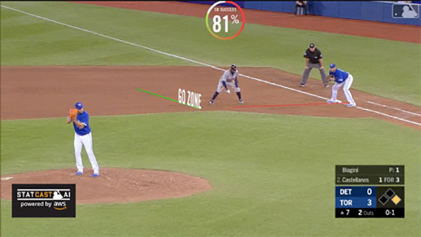
Stolen Base Success Probability provides viewers with a new depth of understanding of the cat and mouse game between the pitcher and the baserunner.

To calculate the Stolen Base Success Probability, AWS used MLB data to train, test, and deploy an ML model that analyzes thousands of data points covering 37 variables that, together, determine whether or not a player safely arrives at second if he attempts to steal. Those variables include the runner’s speed and burst, the catcher’s average pop time to second base, the pitcher’s velocity and handedness, historical stolen base success rates for the runner, batter, and pitcher, along with relevant data about the game context.

We took a 10-fold cross-validation approach to explore a range of classification algorithms, such as logistic regression, support vector machines, random forests, and neural networks, by using historical play data from 2015 to 2018 provided by MLB that corresponds to ~7.3K stolen base attempts with ~5.5K successful stolen bases and ~1.8K runners caught stealing. We applied numerous strategies to deal with the class imbalance, including class weights, custom loss functions, and sampling strategies, and found that the best performing model for predicting the probability of stolen base success was a deep neural network trained on an Amazon Deep Learning (DL) AMI, pre-configured with popular DL frameworks. The trained model was deployed using Amazon SageMaker, which provided the subsecond response times required for integrating predictions into in-game graphics in real-time, and on ML instances that auto-scaled across multiple Availability Zones. For more information, see Deploy trained Keras or TensorFlow models using Amazon SageMaker.

As the player on first base contemplates stealing second, viewers can see his Stolen Base Success Probability score in real-time right on their screens.

MLB offered fans a pilot test and preview of Stolen Base Success Probability during the 2018 postseason. Thanks to feedback from broadcasters and fans, MLB and AWS collaborated during the past offseason to develop an enhanced version with new graphics, improved latency of real-time stats for replays, and a cleaner look. One particular enhancement is the “Go Zone,” the point along the baseline where the player’s chances of successfully making the steal reaches a minimum of 85%.

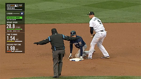
As the player extends his lead towards second, viewers can now see the probability changing dynamically and a jump in his chances of success when he hits the “Go Zone.” After the runner reaches second base, whether he gets called “safe” or “out,” viewers have the opportunity during a replay to see data generated from a variety of factors that may have determined the ultimate outcome, like the runner’s sprint speed and the catcher’s pop time. Plus, that data is color-coded in green, yellow, and red to help fans visualize the factors that played the most significant roles in determining whether or not the player successfully made it to second.

Predicting impact of infield defensive strategies

Over the last decade, there have been few changes in MLB as dramatic as the rise of the infield shift, a “situational defensive realignment of fielders away from their traditional starting points.” Teams use the shift to exploit batted-ball patterns, such as a batter’s tendency to pull batted balls (right field for left-handed hitters and left field for right-handed hitters). As a batter steps up to the plate, the defensive infielders adjust their positions to cover the area where the batter has historically hit the ball into play.

Using Statcast AI data, teams can give their defense an advantage by shifting players to prevent base hits—and teams are employing this strategy more often now than at any other time in baseball history. League-wide shifting rates have increased by 86% over the last three years, up to 25.6% in 2019 from 13.8% in 2016.

AWS and MLB teamed up to employ machine learning to give baseball fans insight into the effectiveness of a shifting strategy. We developed a model to estimate the Shift Impact—the change in a hitter’s expected batting average on ground balls—as he steps up to the plate, using historical data and Amazon SageMaker. As infielders move around the field, the Shift Impact dynamically updates by re-computing the expected batting average with the changing positions of the defenders. This provides a real-time experience for fans.

Using data to quantify the Shift Impact

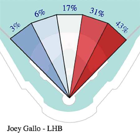
A spray chart can illustrate the tendency batters have in hitting balls towards a particular direction. The chart indicates the percentage at which a player’s batted balls are hit through various sections of the field. The following chart shows the 2018 spray distribution of Joey Gallo’s (from the Texas Rangers) batted balls hit within the infielders’ reach, defined as having a projected distance of less than 200 feet away from home plate. For more information, see Joey Gallo’s current stats on Baseball Savant.

The preceding chart shows the tendency to pull the ball toward right field for Joey Gallo, who hit 74% of his balls to the right of second base in 2018. A prepared defense can take advantage of this observation by overloading the right side of the infield, cutting short the trajectory of the ball and increasing the chance of converting the batted ball into an out.

We estimated the value of specific infield alignments against batters based on their historical batted-ball distribution by taking into account the last three seasons of play, or approximately 60,000 batted balls in the infield. For each of these at-bats, we gathered the launch angle and exit velocity of the batted ball and infielder positions during the pitch, while looking up the known sprint speed and handedness of the batter. While there are many metrics for offensive production in baseball, we chose to use batting average on balls in play—that is, the probability of a ball in play resulting in a base hit.

We calculated how effective a shift might be by estimating the amount by which a specific alignment decreases our offensive measure. After deriving new features, such as the projected landing path of the ball and one-hot encoding the categorical variables, the data was ready for ingestion into various ML frameworks to estimate the probability that a ball in play results in a base hit. From that, we could compute the changes to the probability due to changing infielder alignments.

Using Amazon SageMaker to calculate Shift Impact

We trained ML models on more than 50,000 at-bat samples. We found that the results of a Bayesian search through a hyperparameter optimization (HPO) job using Amazon SageMaker’s Automatic Model Tuning feature over the pre-built XGBoost algorithm on Amazon SageMaker returned the most performant predictions with overall precision of 88%, recall of 88%, and an f1 score of 88% on the validation set of nearly 10,000 events. Launching an HPO job on Amazon SageMaker is as simple as defining the parameters to describe the job, then firing it off to the backend services that manage the core infrastructure (Amazon EC2, Amazon S3, Amazon ECS) to iterate through the defined hyperparameter space efficiently and find the optimal model.

The code snippets shown utilize boto3, the Python API for AWS products and tools. Amazon SageMaker also offers the SageMaker Python SDK, an open source library with several high-level abstractions for working with Amazon SageMaker and popular deep learning frameworks.

Defining the HPO job

We started by setting up the Amazon SageMaker client and defining the tuning job. This specifies which parameters to vary during tuning, along with the evaluation metric we wish to optimize towards. In the following code, we set it to minimize the log loss on the validation set:

import boto3
from sagemaker import get_execution_role
from sagemaker.amazon.amazon_estimator import get_image_uri

sm_client = boto3.Session().client('sagemaker')
xgboost_image = get_image_uri(boto3.Session().region_name, 'xgboost')
role = get_execution_role()

tuning_job_config = {
    "ParameterRanges": {
      "CategoricalParameterRanges": [],
      "ContinuousParameterRanges": [
        {
          "MaxValue": "1",
          "MinValue": "0",
          "Name": "eta"
        },
        {
          "MaxValue": "2",
          "MinValue": "0",
          "Name": "alpha"
        },
      ],
      "IntegerParameterRanges": [
        {
          "MaxValue": "10",
          "MinValue": "1",
          "Name": "max_depth"
        },
      ]
    },
    "ResourceLimits": {
      "MaxNumberOfTrainingJobs": 100,
      "MaxParallelTrainingJobs": 10
    },
    "Strategy": "Bayesian",
    "HyperParameterTuningJobObjective": {
      "MetricName": "validation:logloss",
      "Type": "Minimize"
    }
  }
 
training_job_definition = {
    "AlgorithmSpecification": {
      "TrainingImage": xgboost_image,
      "TrainingInputMode": "File"
    },
    "InputDataConfig": [
      {
        "ChannelName": "train",
        "CompressionType": "None",
        "ContentType": "csv",
        "DataSource": {
          "S3DataSource": {
            "S3DataDistributionType": "FullyReplicated",
            "S3DataType": "S3Prefix",
            "S3Uri": s3_input_train # path to training data
          }
        }
      },
      {
        "ChannelName": "validation",
        "CompressionType": "None",
        "ContentType": "csv",
        "DataSource": {
          "S3DataSource": {
            "S3DataDistributionType": "FullyReplicated",
            "S3DataType": "S3Prefix",
            "S3Uri": s3_input_validation # path to validation data
          }
        }
      }
    ],
    "OutputDataConfig": {
      "S3OutputPath": s3_output # outpath path for model artifacts
    },
    "ResourceConfig": {
      "InstanceCount": 2,
      "InstanceType": "ml.c4.2xlarge",
      "VolumeSizeInGB": 10
    },
    "RoleArn": role,
    "StaticHyperParameters": {
      "eval_metric": "logloss",
      "objective": "binary:logistic",
      "rate_drop": "0.3",
      "tweedie_variance_power": "1.4",
    },
    "StoppingCondition": {
      "MaxRuntimeInSeconds": 43200
    }
}

Launching the HPO job

With the tuning job defined in the Python dictionary above, we now submit it to the Amazon SageMaker client, which then automates the process of launching EC2 instances with containers optimized to run XGBoost from ECS. See the following code:

sm_client.create_hyper_parameter_tuning_job(HyperParameterTuningJobName = "tuning_job_name",
                                            HyperParameterTuningJobConfig = tuning_job_config,
                                            TrainingJobDefinition = training_job_definition)

During the game, we can analyze a given batter with his most recent at-bats and run those events through the model for all infielder positions as laid out on a grid. Since the amount of compute required for inference increases geometrically as the size of each grid cell is reduced, we adjusted the size to reach a balance between the resolution required for meaningful predictions and compute time. For example, consider a shortstop that shifts over to his left. If he moves over by only one foot, there will be a negligible effect on the outcome of a batted ball. However, if he repositions himself 10 feet to his left, that can very well put himself in a better position to field a ground ball pulled to right field. Examining all at-bats in our dataset, we found such a balance on a grid composed of 10-foot by 10-foot cells, accounting for more than 10,000 infielder configurations.

The process of obtaining the best performing model from the HPO job and deploying to production follows in the next section. Due to the large number of calls required for real-time inference, the results of the model are prepopulated into a lookup table that provides the relevant predictions during a live game.

Deploying the most performant model

Each tuning job launches a number of training jobs, from which the best model is selected according to the criteria defined earlier when configuring the HPO. From Amazon SageMaker, we first pull the best training job and its model artifacts. These are stored in the S3 bucket from which the training and validation datasets were pulled. See the following code:

# get best model from HPO job
best_training_job = smclient.describe_hyper_parameter_tuning_job(
    HyperParameterTuningJobName=tuning_job_name)['BestTrainingJob']
info = smclient.describe_training_job(TrainingJobName=best_training_job['TrainingJobName'])
model_name = best_training_job['TrainingJobName'] + '-model'
model_data = info['ModelArtifacts']['S3ModelArtifacts']

Next, we refer to the pre-configured container optimized to run XGBoost models and link it to the model artifacts of the best-trained model. Once this model-container pair is created on our account, we can configure an endpoint with the instance type, number of instances, and traffic splits (for A/B testing) of our choice:

create_model_response = sm_client.create_model(
    ModelName = model_name,
    ExecutionRoleArn = role,
    PrimaryContainer = {
        'Image': xgboost_image,
        'ModelDataUrl': model_data})

# create endpoint configuration
endpoint_config_name = model_name+'-endpointconfig'
create_endpoint_config_response = sm_client.create_endpoint_config(
    EndpointConfigName = endpoint_config_name,
    ProductionVariants=[{
        'InstanceType':'ml.m5.2xlarge',
        'InitialVariantWeight':1,
        'InitialInstanceCount':1,
        'ModelName':model_name,
        'VariantName':'AllTraffic'}])

# create endpoint
endpoint_name = model_name+'-endpoint'
create_endpoint_response = smclient.create_endpoint(
EndpointName=endpoint_name,
EndpointConfigName=endpoint_config_name)
resp = sm_client.describe_endpoint(EndpointName=endpoint_name)
status = resp['EndpointStatus']

print("Arn: " + resp['EndpointArn'])
print(create_endpoint_response['EndpointArn'])

Inference from the endpoint

The Amazon SageMaker runtime client makes predictions from the model, and sends a request to the endpoint hosting the model container on an EC2 instance and returns the output. We can configure entry points of the endpoint for custom models and data processing steps:

# invoke endpoint
runtime_client = boto3.client('runtime.sagemaker')
random_payload = np.array2string(np.random.random(num_features), separator=',', max_line_width=np.inf)[1:-1]
response = runtime_client.invoke_endpoint(EndpointName=endpoint_name, Body=random_payload)
prediction = response['Body'].read().decode("utf-8")
print(prediction) 

With all of the predictions for a given batter and infielder configurations, we then average the probability of a base hit returned from the model stored in the lookup table and subtract the expected batting average for the same sample of batted balls. The resulting metric is the Shift Impact.

Matchup Analysis

In interleague games, where teams from the American and National leagues compete against each other, many batters face pitchers they have never seen before. Estimating outcomes in interleague games is difficult because there is limited relevant historical data. AWS worked with MLB to group similar pitchers together to gain insight on how the batter has historically performed against similar pitchers. We took a machine learning approach, which allowed us to combine the domain knowledge of experts with data comprised of hundreds of thousands of pitches to find additional patterns we could use to identify similar pitchers.

Modeling

Taking inspiration from the field of recommendation systems, in which the matching problem is typically solved by computing a user’s inclination towards a product, here we seek to determine the interaction between a pitcher and batter. There are many algorithms appropriate to building recommenders, but few that allow us to then cluster like items that are put into the algorithm. Neural networks shine in this area. End layers in a neural network architecture can be interpreted as numerical representations of the input data, whether it be an image or a pitcher ID. Given input data, its associated numerical representation–or embedding–can be compared against the embeddings of other input items. Those embeddings that lie near each other are similar, not just in this embedding space, but also in interpretable characteristics. For example, we expect handedness to play a role in defining which pitchers are similar. This approach to recommendation systems and clustering items is known as deep matrix factorization.

Deep matrix factorization accounts for nonlinear interactions between a pair of entities, while also mixing in the techniques of content-based and collaborative filtering. Rather than working solely with a pitcher-batter matrix, as in matrix factorization, we build a neural network that aligns each pitcher and batter with their own embedding and then pass them through a series of hidden layers that are trained towards predicting the outcome of a pitch. In addition to the collaborative nature of this architecture, additional contextual data is included for each pitch such as the count, number of runners on base, and the score.

The model is optimized against the predicted outcome of each pitch, including both the pitch characteristics (slider, changeup, fastball, etc.) and the outcome (ball, single, strike, swinging strike, etc.). After training a model on this classification problem, the end layer of the pitcher ID input is extracted as the embedding for that particular pitcher.

Results

As a batter steps up to the plate against a pitcher he hasn’t faced before, we search for the nearest embeddings to that of the opposing pitcher and calculate the on-base plus slugging percentage (OPS) against that group of pitchers. To see the results in action, see 9/11/19: FSN-Ohio executes OPS comparison.

Summary

MLB uses cloud computing to create innovative experiences that introduce additional ways for fans to experience baseball. With Stolen Base Success Probability, Shift Impact, and Pitcher Similarity Match-up Analysis, MLB provides compelling, real-time insight into what’s happening on the field and a greater connection to the context that builds the unique drama of the game that fans love.

This postseason, fans will have many opportunities to see stolen base probability in action, the potential effects of infield alignments, and launch into debates with friends about what makes pitchers similar.

Fans can expect to see these new stats in live game broadcasts with partners such as ESPN and MLB Network. Plus, other professional sports leagues including the NFL and Formula 1 have selected AWS as their cloud and machine learning provider of choice.

You can find full, end-to-end examples of implementing an HPO job on Amazon SageMaker at the AWSLabs GitHub repo. If you’d like help accelerating your use of machine learning in your products and processes, please contact the Amazon ML Solutions Lab program.

About the Authors

Hussain Karimi is a data scientist at the Amazon ML Solutions Lab, where he works with AWS customers to develop machine learning models that uncover unique insights in various domains.

Travis Petersen is a Senior Data Scientist at MLB Advanced Media and an adjunct professor at Fordham University.

Priya Ponnapalli is a principal scientist and manager at Amazon ML Solutions Lab, where she helps AWS customers across different industries accelerate their AI and cloud adoption.